Learning Calculus With Python

Learning calculus with Python can be an incredibly rewarding experience, particularly when it comes to understanding two key concepts-

1. Differentiation
2. Integration

These fundamental operations are at the heart of many machine learning algorithms, optimization problems, and data science tasks.

Python provides a way to not only perform differentiation and integration but also visualize their effects, making abstract concepts more tangible and easier to grasp.

In this article, we’ll explore how Python can be used to learn calculus and visualize these concepts, equipping you with the tools to apply them in practical scenarios.

A Glimpse of Learning Calculus With Python

Understand & Perform Differentiation in Python

Differentiation is a core calculus concept that measures how a function changes at any given point.

In simpler terms, it provides us with the slope of the curve at a particular point.

Differentiation is widely used in areas like machine learning, which helps optimize models by minimizing error functions, and in physics, where it tracks rates of change such as velocity and acceleration.

Python offers several ways to compute derivatives, both symbolically and numerically.

The SymPy library is a great tool for symbolic differentiation.

SymPy allows us to express functions in mathematical terms and compute their derivatives with ease.

Take a simple example of the function f(x) = x^2 + 2x + 1:

import sympy as sp
x = sp.symbols('x')
f = x**2 + 2*x + 1
derivative = sp.diff(f, x)
print(derivative)

Output:

The derivative, 2x + 2, tells us how the function’s rate of change varies at any point.

SymPy makes it easy to calculate derivatives for much more complex functions as well. However, for working with data points or real-world measurements, numerical differentiation might be more practical. NumPy’s gradient() function is perfect for this.

Consider the following example where we approximate the derivative of f(x) = x^2 at discrete points:

import numpy as np
x_vals = np.linspace(0, 10, 100)
y_vals = x_vals**2
dydx = np.gradient(y_vals, x_vals)

This gives us the rate of change of y = x^2 at each point in the x_vals array. But to truly understand the significance of this derivative, we can visualize both the original function and its derivative using Matplotlib.

Visualization provides a clear picture of how the function’s slope evolves across its domain:

import matplotlib.pyplot as plt
plt.plot(x_vals, y_vals, label="f(x) = x^2")
plt.plot(x_vals, dydx, label="Derivative of f(x)")
plt.legend()
plt.show()

Output:

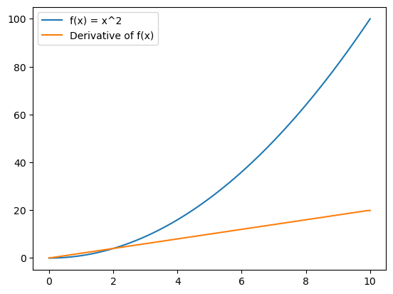
The plot visually captures the behavior of both the function and its derivative, allowing us to observe how the curve steepens as x increases.

Understand & Perform Integration in Python: Accumulating Quantities

While differentiation gives us the rate of change, integration is the reverse operation.

It calculates the total accumulation of a quantity over a given interval, which is often visualized as the area under a curve. Integration is essential in areas such as probability, where it helps in calculating probabilities over continuous intervals, and in physics for computing quantities like displacement from velocity.

Like differentiation, integration in Python can be performed symbolically or numerically.

SymPy once again comes in handy for symbolic integration.

For example, to compute the indefinite integral of f(x) = x^2 + 2x + 1, you can write:

integral = sp.integrate(f, x)
print(integral)

The result x^3/3 + x^2 + x represents the antiderivative of f(x). SymPy also supports definite integrals, allowing you to compute the exact area under the curve between two points:

definite_integral = sp.integrate(f, (x, 0, 5))
print(definite_integral)

In practice, numerical integration is often more useful, especially when working with data. SciPy’s quad() function provides an efficient way to compute numerical integrals. Here’s how to integrate f(x) = x^2 from 0 to 5 numerically:

from scipy import integrate
result, _ = integrate.quad(lambda x: x**2, 0, 5)
print(result)

This gives a numerical approximation of the area under f(x) = x^2 between 0 and 5. To fully appreciate what the integral represents, let’s visualize the function and the shaded area that corresponds to the integral:

plt.plot(x_vals, y_vals, label="f(x) = x^2")
plt.fill_between(x_vals, y_vals, alpha=0.3)
plt.legend()
plt.show()

Output:

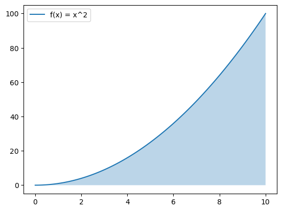
The plot clearly shows the curve and the shaded region beneath it, helping to solidify the concept of integration as the area under a curve. By using Python’s visualization capabilities, we can more easily grasp how integration works and see its applications in various contexts.

Learning calculus through Python is practical as well as empowering.

With Python’s robust libraries, you can compute and visualize both differentiation and integration, making abstract mathematical concepts more concrete. Whether you are working on machine learning models, data analysis, or scientific research, Python simplifies the application of these powerful calculus tools.