Zeta Function in Python

The Zeta function encompasses a family of important mathematical functions, primarily including the Riemann Zeta function and the Hurwitz Zeta function. The Riemann Zeta function has an important part to play in understanding how prime numbers are distributed.

The Hurwitz Zeta function generalizes the Riemann Zeta function, allowing it to accommodate a wider range of applications in fields like probability theory, quantum physics, and algebraic geometry. This tutorial will discuss how to make use of the zeta function in Python.

The Riemann Zeta Function in Python

The Riemann Zeta function is significant in number theory and is denoted as \zeta(s). It is defined by the infinite series:

\zeta(s) = \sum_{n=1}^{\infty} \frac{1}{n^s}

where s is a complex number. One important application of the Riemann Zeta function is in investigating the distribution of prime numbers.

The famous Riemann Hypothesis states that the non-trivial zeros of the zeta function lie on the critical line where \Re(s) = \dfrac{1}{2}.

Using SciPy to compute the Riemann Zeta Function in Python

The scipy library in Python has an implementation of the Riemann Zeta function.

This function can be accessed as scipy.special.zeta and is used to evaluate the zeta function for real and complex values of s.

Here’s a code example of the scipy in action:

import scipy.special as sp

# Riemann Zeta function using SciPy
s = 2  # Example value for s
riemann_zeta = sp.zeta(s)
print(f"Riemann Zeta function at s = {s}: {riemann_zeta}")

Output:

For s = 2, the output will be:

This value corresponds to the well-known result \zeta(2) = \dfrac{\pi^2}{6}, which is central in number theory.

The Hurwitz Zeta Function in Python

The Hurwitz Zeta function incorporates an additional parameter q, and is defined as:

\zeta(s, q) = \sum_{n=0}^{\infty} \frac{1}{(n + q)^s}

where s is a complex number and q is a real number with q > 0.

For the special case (when q = 1), the function becomes the Riemann Zeta function.

Just like with the Riemann Zeta function, the Hurwitz Zeta function can be computed using the scipy.special.zeta function.
This time, we will need to supply two arguments, s and q.

See the code example below for how to call the scipy.special.zeta function:

import scipy.special as sp

# Hurwitz Zeta function using SciPy
s = 2  # Example value for s
q = 1.5  # Example value for q
hurwitz_zeta = sp.zeta(s, q)
print(f"Hurwitz Zeta function at s = {s}, q = {q}: {hurwitz_zeta}")

Output:

For s = 2 and q = 1.5, the output will be:

This computation reflects the generalized form of the zeta function, incorporating the shift parameter q, showcasing how the Hurwitz Zeta function extends the applicability of its Riemann counterpart.

Visualizing the Zeta Function with Hurwitz Generalization

The Riemann Zeta function and its generalization, the Hurwitz Zeta function, provide insights into number theory and mathematical analysis.

To visualize the behavior of these functions when s is real, we can plot the series for different values of the parameter q, showcasing the convergence patterns for each case.

The Riemann Zeta function is given by the series:

\zeta(s) = \sum_{n=1}^{\infty} \frac{1}{n^s}

Expanding this:

\zeta(s) = \frac{1}{1^s} + \frac{1}{2^s} + \frac{1}{3^s} + \frac{1}{4^s} + \dots

This series starts at n = 1 and sums over all positive integers.

For q = 2, 3, 5, the Hurwitz Zeta function shifts the series by those values:

\zeta(s, 2) = \sum_{n=0}^{\infty} \frac{1}{(n + 2)^s} \zeta(s, 3) = \sum_{n=0}^{\infty} \frac{1}{(n + 3)^s} \zeta(s, 5) = \sum_{n=0}^{\infty} \frac{1}{(n + 5)^s}

Expanding these, we get the infinite series:

\zeta(s, 2) = \frac{1}{2^s} + \frac{1}{3^s} + \frac{1}{4^s} + \frac{1}{5^s} + \dots \zeta(s, 3) = \frac{1}{3^s} + \frac{1}{4^s} + \frac{1}{5^s} + \frac{1}{6^s} + \dots \zeta(s, 5) = \frac{1}{5^s} + \frac{1}{6^s} + \frac{1}{7^s} + \frac{1}{8^s} + \dots

We can now visualize how the Riemann Zeta function (q = 1) and Hurwitz Zeta functions (q = 2, 3, 5) behave for different real values of s using Python. These plots will provide insights into how the growth of these functions changes as q increases and highlight the critical vertical asymptotes at s = 1.

To compute the values of the Riemann and Hurwitz Zeta functions, we use mpmath instead of scipy. scipy.special.zeta has known limitations when computing values for real numbers between 0 and 1 when the value of q is specified.

For instance, calling scipy.special.zeta(1/2, 1) incorrectly returns NaN due to how the Hurwitz Zeta function is defined in scipy, even though the correct value should be approximately -1.46.

In contrast, mpmath supports the full analytic continuation of the zeta function and provides high-precision results, making it more reliable for computations across the entire range of real and complex inputs.

import numpy as np
import matplotlib.pyplot as plt
from mpmath import zeta

def calculate_zeta_values(s_values, q=1):
    return [zeta(s, q) for s in s_values]

def plot_zeta_function(ax, s_neg, s_pos, q, color, label):
    # Calculate the zeta values for both subdomains
    zeta_neg = calculate_zeta_values(s_neg, q)
    zeta_pos = calculate_zeta_values(s_pos, q)
    
    # Plot the values for both subdomains with the same label
    ax.plot(s_neg, zeta_neg, color=color)
    ax.plot(s_pos, zeta_pos, color=color, label=label)

    # Add asymptote at s = 1
    ax.axvline(x=1, color='gray', linestyle='--')  # Asymptote at s = 1
    ax.set_xlabel('s (Real part)')
    ax.set_ylabel(r'$\zeta(s, q)$')
    ax.legend()
    ax.grid(True)
    ax.set_ylim(-10, 10)  # Adjust y-limits for better visualization

def visualize_zeta_functions():
    # Define real part of s, avoiding s = 1 and close values
    s_neg = np.linspace(0.1, 0.9, 500)  # From 0.1 to 0.9
    s_pos = np.linspace(1.1, 5, 500)    # From 1.1 to 5
    
    # Initialize a 2x2 grid of subplots
    fig, axs = plt.subplots(2, 2, figsize=(14, 10))

    # Plot Riemann Zeta function (q=1)
    plot_zeta_function(axs[0, 0], s_neg, s_pos, q=1, color='blue', label=r'Riemann $\zeta(s)$')

    # Plot Hurwitz Zeta function for q=2, q=3, q=5
    plot_zeta_function(axs[0, 1], s_neg, s_pos, q=2, color='orange', label=r'Hurwitz $\zeta(s, 2)$')
    plot_zeta_function(axs[1, 0], s_neg, s_pos, q=3, color='green', label=r'Hurwitz $\zeta(s, 3)$')
    plot_zeta_function(axs[1, 1], s_neg, s_pos, q=5, color='red', label=r'Hurwitz $\zeta(s, 5)$')

    # Set titles for each subplot
    axs[0, 0].set_title('Riemann Zeta Function (q=1)')
    axs[0, 1].set_title('Hurwitz Zeta Function (q=2)')
    axs[1, 0].set_title('Hurwitz Zeta Function (q=3)')
    axs[1, 1].set_title('Hurwitz Zeta Function (q=5)')

    # Adjust layout to prevent overlap
    plt.tight_layout()
    
    # Show the plot
    plt.show()

# Visualize the plots
visualize_zeta_functions()

The provided script visualizes both the Riemann Zeta function and the Hurwitz Zeta function for different values of the parameter q. The function values are plotted for two distinct subdomains: one where 0 < s < 1. These ranges were chosen to avoid the singularity that occurs at s = 1, where the Zeta function diverges. The mpmath library is used to compute the Zeta function values for both the Riemann case (q = 1) and the Hurwitz cases with (q = 2, 3, 5). Each function is plotted in a different subplot for clear comparison.

The reason for splitting the real values of s into two subdomains is to properly handle the asymptote at s=1. Without dividing the range, matplotlib would attempt to connect the values on both sides of s=1, which would cause the plot to incorrectly smooth over the singularity and misrepresent the behavior of the function.

By splitting the domain, the plot ensures that the asymptote is clearly visible, and a vertical dashed line is added at s=1 to indicate the divergence, ensuring proper visualization of the Zeta function’s distinct behavior in each subdomain.

Output:

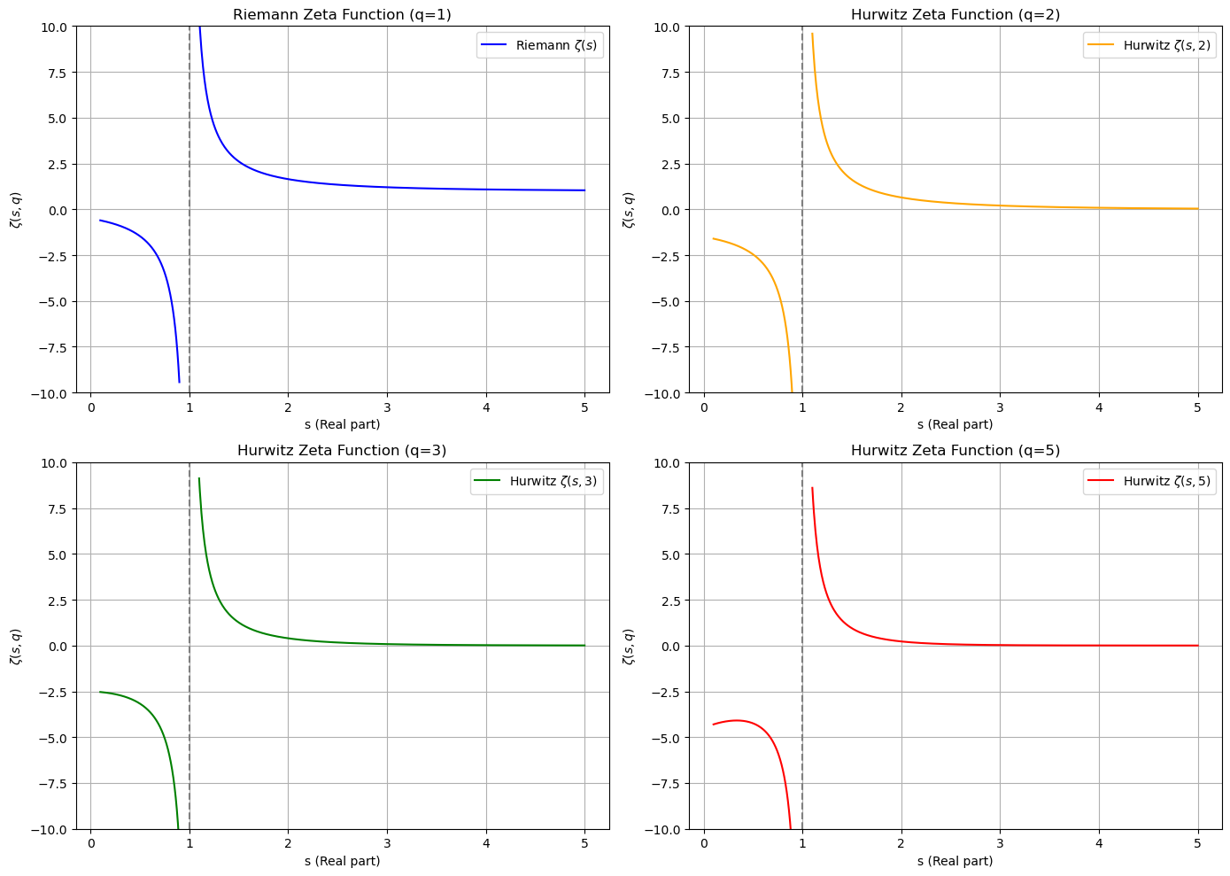
The visualizations of the Riemann and Hurwitz Zeta functions with different q-values highlight several key insights.

A vertical asymptote at s = 1 is visible in all plots, indicating the point where the Zeta function becomes undefined.

This asymptotic behavior is consistent across both the Riemann and Hurwitz Zeta functions. In the range 0 < s < 1, the function rapidly decreases to negative infinity as s approaches 1 from the left, with the rate of decrease slightly varying based on q.

In conclusion, the Python libraries scipy and mpmath provide accessible implementations for both the Riemann and Hurwitz Zeta functions.

These tools allow users to explore complex mathematical concepts such as prime distribution and generalized Zeta functions straightforwardly.